The Log-Ratio Scale: How to Calculate Outperformance

In relative-value or statistical-arbitrage work, the first core problem is this: how do you measure, precisely and without bias, whether asset A is truly outperforming asset B?

Simple division looks intuitive. It already embeds an asymmetry bias that can poison every downstream indicator.

Why simple division is wrong

Use an extreme mathematical example to dismantle the flaw in the simple ratio.

Suppose we compare asset A and asset B. Both start at $100. Initial ratio: 100 / 100 = 1.0.

Then the market moves violently.

• Scenario 1 (A surges): A doubles to $200 while B stays at $100. A/B becomes 200 / 100 = 2.0. Change in ratio: +1.0.
• Scenario 2 (A crashes): A is cut in half to $50 while B stays at $100. A/B becomes 50 / 100 = 0.5. Change in ratio: −0.5.

Stop and think about that result. In real investing, A “doubling (+100%)” and A “losing half (−50%)” are equal in absolute magnitude and market impact. They are exact mirrors.

But with a simple ratio, the upward move produces +1.0 while the downward move produces only −0.5.

Statistically, this distribution is right-skewed. It is not a symmetric bell curve: the right tail can stretch without bound (the ratio can grow indefinitely), while the left side is hard-capped at 0 (prices cannot go negative).

What goes wrong? If you compute the standard deviation or mean of that A/B series, the results skew upward. Your model systematically overweights rallies and underestimates declines. If your strategy closes at “2 standard deviations from the mean,” this asymmetry makes you exit too early in bull runs and wait forever for a stop in bear markets.

To fix that distributional bias, you need a different tool.

How the natural logarithm restores symmetry

Quant engineers introduce the natural logarithm $\ln$ (logarithm with Euler’s number $e$ as base).

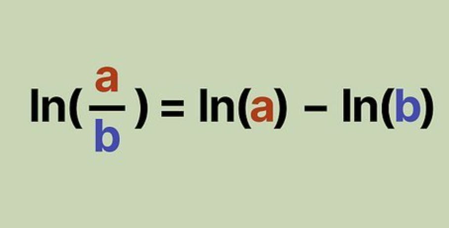
By basic log properties, the log of a quotient decomposes into a difference of logs:

$$ \ln\left(\frac{A}{B}\right) = \ln(A) - \ln(B) $$

Apply the same extreme example:

• Initial: $\ln(100/100) = \ln(1) = 0$
• Doubling: $\ln(200/100) = \ln(2.0) \approx +0.693$
• Halving: $\ln(50/100) = \ln(0.5) \approx -0.693$

Perfect symmetry. Whether the asset doubles or is cut in half, the log-ratio produces values of equal magnitude and opposite sign (+0.693 and −0.693). That means Ln(A/B) truly and objectively represents the cumulative return difference between the two assets.

Under continuous compounding, the log-difference of prices is the asset’s true rate of return. This removes skew from extreme values and leaves a distribution that closely approximates normality: a clean signal source that statistical tools (Z-scores, percentile ranks, mean-reversion models) can process safely.

Symmetry is solved. Live trading hits a second problem: absolute volatility cannot share one fixed threshold across assets.

The volatility gap: why convert to 0–100

With a symmetric Ln(A/B) in hand, the first mathematical problem is solved. The moment you go live, a second fatal issue appears: absolute volatility differs enormously across asset sectors.

In the Macro-Rotational Portfolio, we monitor dozens of pairs.

• SMH / XLK (semiconductors vs broad tech): both are high-beta; the log-spread is wildly volatile.
• XLP / SPY (consumer staples vs the market): an extremely defensive pair; the log-spread usually moves slowly.

If you use one fixed absolute threshold (say $\ln$ spread > 0.05) as a system-wide entry rule, it becomes a catastrophe. For semis, that level may be ordinary daily noise. For staples, it may not trigger once in a decade.

To strip out absolute volatility, apply a second mathematical standardization: convert the log-ratio into a rolling percentile rank (0–100).

Standard transformation logic used in the system core:

# Macro-Rotational Portfolio: core signal generator
import numpy as np
import pandas as pd

def generate_log_spread_signal(price_A: pd.Series, price_B: pd.Series, window: int = 10) -> pd.Series:
    """
    Compute the rolling percentile rank of the log-spread
    """
    # Step 1: compute the perfectly symmetric log-ratio (Log-Spread)
    log_spread = np.log(price_A / price_B)
    
    # Step 2: compute the percentile rank over the past 10 days (0 to 100)
    # Use a rolling window to strip out absolute volatility and extract only relative extremeness
    percentile_rank = log_spread.rolling(window).apply(
        lambda x: pd.Series(x).rank(pct=True).iloc[-1] * 100, 
        raw=False
    )
    
    return percentile_rank

What does this 0–100 score mean?

When percentile_rank hits 95, it no longer represents a specific price spread. It represents an extreme state: “The degree to which semiconductors outperformed the broad market today beats 95% of the days over the past two weeks (10 trading days). This is the most extreme Top 5% of strength.”

That step puts every asset on the same field. Whether it is volatile crypto or quiet bonds, a momentum rank above 95 means capital is flooding in at an abnormal pace. What we capture is this short-window “relative momentum impulse.”

Window length can decide whether the strategy survives.

Why 10 days, not 20 or 50

In quantitative backtesting, window size often decides whether a strategy lives or dies. Why choose 10 days (two weeks) as the rolling percentile window instead of the more common 20 days (one month) or 50 days?

It comes from observations of institutional order flow.

In modern markets, rebalancing by macro hedge funds and passive ETFs tends to be highly impulsive. When a new macro narrative appears (AI capex beating expectations, or an inflation print blowing out), institutional cross-sector rotation usually completes concentrated position-building within 1 to 2 weeks.

• Window too long (e.g. 50 days): the signal becomes sluggish. By the time the 50-day percentile reaches 90, institutional accumulation is long over and the move is in its tail, or about to reverse. You enter just in time to become exit liquidity for distribution.
• Window too short (e.g. 3 days): the signal drowns in white noise. One day of programmatic selling by a large player whipsaws the percentile, and the system emits many false signals.

10 days (two full trading weeks) is a balance point rigorously validated by walk-forward optimization. It is long enough to contain a complete theme incubation window, and it fires when capital momentum is fiercest: trend confirmed, not yet exhausted.

Turning noise into a comparable signal

Retail traders stare at candlesticks on TradingView, trying to find order in chaos by eye. That is close to staring at wave shapes in a storm and trying to predict the next second of wind.

The Log-Spread Indicator is the sonar we built instead. Through the natural logarithm, we eliminate distribution asymmetry bias. Through the 10-day rolling percentile, we filter interference from differing asset volatilities. Unpredictable price noise becomes a pure, stationary, highly comparable mathematical signal.

That is the bedrock on which the Macro-Rotational Portfolio runs. In quant work, the sharpest weapon is rarely a complicated neural network. It is a thorough mathematical understanding of the data’s underlying characteristics.

Source: Cross-Asset Pricing: The Mathematical Brute Force of the Log-Ratio